핸즈온 머신러닝[2] 머신러닝 프로젝트 처음부터 끝까지(3)
https://www.youtube.com/watch?v=8-miINfxCm4&list=PLJN246lAkhQjX3LOdLVnfdFaCbGouEBeb&index=9
모델 선택과 훈련
1. 훈련 세트에서 훈련하고 평가하기
from sklearn.linear_model import LinearRegression

lin_reg = LinearRegression()
lin_reg.fit(housing_prepared, housing_labels)
파라미터: housing_prepared 트레이닝셋, housing_labels 타깃값
# 훈련 샘플 몇 개를 사용해 전체 파이프라인을 적용해 보겠습니다
some_data = housing.iloc[:5]
some_labels = housing_labels.iloc[:5]
some_data_prepared = full_pipeline.transform(some_data)

print("예측:", lin_reg.predict(some_data_prepared))
예측: [ 85657.90192014 305492.60737488 152056.46122456 186095.70946094 244550.67966089]
loc (location) 함수: 데이터프레임의 행이나 컬럼에 label이나 boolean array로 접근
iloc (integer location) 함수: 데이터프레임의 행이나 컬럼에 인덱스 값으로 접근
print("레이블:", list(some_labels))레이블: [72100.0, 279600.0, 82700.0, 112500.0, 238300.0]
some_data_prepared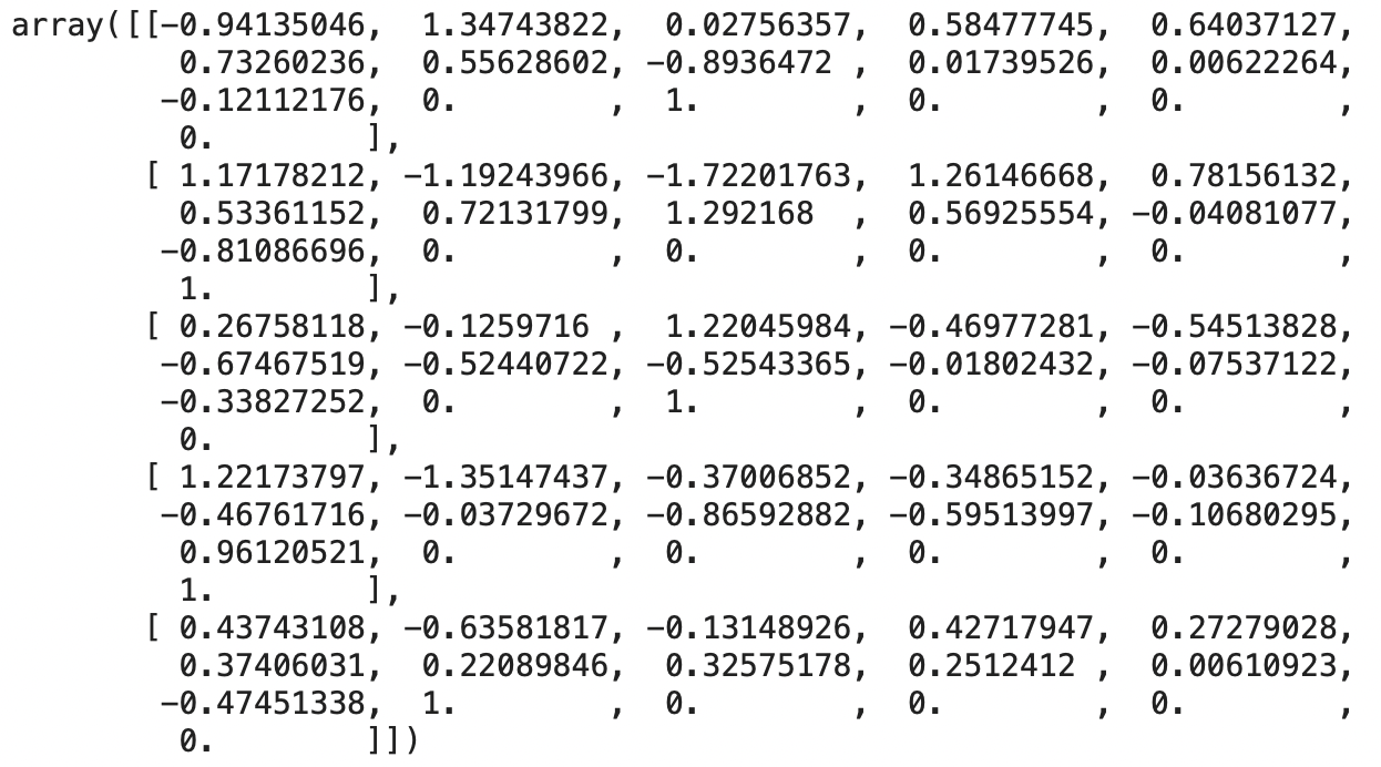
from sklearn.metrics import mean_squared_error

housing_predictions = lin_reg.predict(housing_prepared)
lin_mse = mean_squared_error(housing_labels, housing_predictions)
lin_rmse = np.sqrt(lin_mse)
lin_rmse
68627.87390018745
mse: mean squared error
rmse: root mean squared error
from sklearn.metrics import mean_absolute_error

lin_mae = mean_absolute_error(housing_labels, housing_predictions)
lin_mae

lin_reg.score(housing_prepared, housing_labels)
# score 값 -> r-squared 값
49438.66860915802
0.6481624
mae: mean absolute error
from sklearn.tree import DecisionTreeRegressor

tree_reg = DecisionTreeRegressor(random_state=42)
tree_reg.fit(housing_prepared, housing_labels)
Decision Tree: 결정 트리
Regressor: 회귀 모델
Classifier: 분류 모델
housing_predictions = tree_reg.predict(housing_prepared)
tree_mse = mean_squared_error(housing_labels, housing_predictions)
tree_rmse = np.sqrt(tree_mse)
tree_rmse

tree_reg.score(housing_prepared, housing_labels)
rmse: 0.0 -> 완벽하게 타깃값을 맞췄음 (과대적합)
score: 1.0
2. 교차 검증을 사용한 평가
교차검증: cross validation
from sklearn.model_selection import cross_val_score

scores = cross_val_score(tree_reg, housing_prepared, housing_labels,
                         scoring="neg_mean_squared_error", cv=10)
tree_rmse_scores = np.sqrt(-scores)
cross_val_score -> k-fold
cv: fold 수
neg_mean_squared_error: 음수 MSE
def display_scores(scores):
    print("점수:", scores)
    print("평균:", scores.mean())
    print("표준 편차:", scores.std())

display_scores(tree_rmse_scores)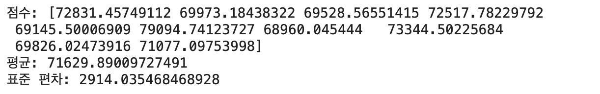
lin_scores = cross_val_score(lin_reg, housing_prepared, housing_labels,
                             scoring="neg_mean_squared_error", cv=10)
lin_rmse_scores = np.sqrt(-lin_scores)
display_scores(lin_rmse_scores)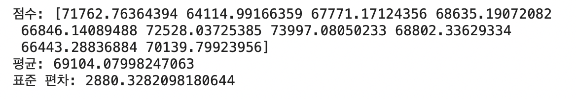
from sklearn.ensemble import RandomForestRegressor

forest_reg = RandomForestRegressor(n_estimators=100, random_state=42)
forest_reg.fit(housing_prepared, housing_labels)
트리 모델을 사용한 앙상블 모델: 결정트리 100개를 만들어서 각각을 훈련한 다음, 트리의 결과를 평균을 내서 사용
중복을 허용해서 random으로 샘플을 뽑음
housing_predictions = forest_reg.predict(housing_prepared)
forest_mse = mean_squared_error(housing_labels, housing_predictions)
forest_rmse = np.sqrt(forest_mse)
forest_rmse
18603.515021...
from sklearn.model_selection import cross_val_score

forest_scores = cross_val_score(forest_reg, housing_prepared, housing_labels,
                                scoring="neg_mean_squared_error", cv=10)
forest_rmse_scores = np.sqrt(-forest_scores)
display_scores(forest_rmse_scores)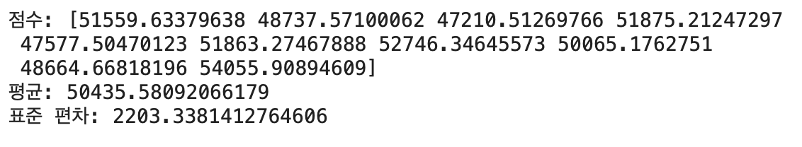
scores = cross_val_score(lin_reg, housing_prepared, housing_labels, scoring="neg_mean_squared_error", cv=10)
pd.Series(np.sqrt(-scores)).describe()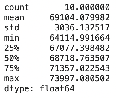
from sklearn.svm import SVR

svm_reg = SVR(kernel="linear")
svm_reg.fit(housing_prepared, housing_labels)
housing_predictions = svm_reg.predict(housing_prepared)
svm_mse = mean_squared_error(housing_labels, housing_predictions)
svm_rmse = np.sqrt(svm_mse)
svm_rmse
Support vector machine
SVR: Support vector machine Regressor
SVC: Support vector machine Classifier
모델 세부 튜닝
1. 그리드 탐색
from sklearn.model_selection import GridSearchCV
param_grid = [
# 12(=3×4)개의 하이퍼파라미터 조합을 시도합니다.
{'n_estimators': [3, 10, 30], 'max_features': [2, 4, 6, 8]},
# bootstrap은 False로 하고 6(=2×3)개의 조합을 시도합니다.
{'bootstrap': [False], 'n_estimators': [3, 10], 'max_features': [2, 3, 4]},
]
forest_reg = RandomForestRegressor(random_state=42)
# 다섯 개의 폴드로 훈련하면 총 (12+6)*5=90번의 훈련이 일어납니다.
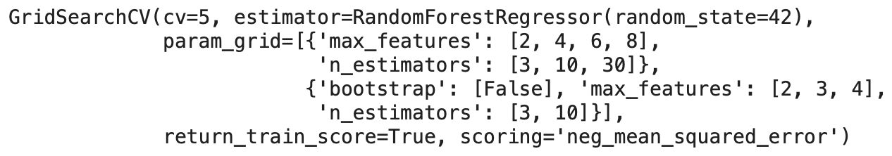
grid_search = GridSearchCV(forest_reg, param_grid, cv=5,
scoring='neg_mean_squared_error',
return_train_score=True)
grid_search.fit(housing_prepared, housing_labels)GridSearchCV(model, param_grid=param_grid,cv=cv,scoring='')
n estimator: 랜덤 포레스트 안에 만들어지는 의사결정나무 갯수. 트리가 많아지면 속도가 느려지고 너무 트리가 크면 오히려 정확도가 낮아진다.
grid_search.best_params_{'max_features': 8, 'n_estimators': 30}
grid_search.best_estimator_RandomForestRegressor(max_features=8, n_estimators=30, random_state=42)
cvres = grid_search.cv_results_
for mean_score, params in zip(cvres["mean_test_score"], cvres["params"]):
    print(np.sqrt(-mean_score), params)
pd.DataFrame(grid_search.cv_results_)2. 랜덤 탐색
from sklearn.model_selection import RandomizedSearchCV
from scipy.stats import randint

param_distribs = {
        'n_estimators': randint(low=1, high=200),
        'max_features': randint(low=1, high=8),
    }

forest_reg = RandomForestRegressor(random_state=42)
rnd_search = RandomizedSearchCV(forest_reg, param_distributions=param_distribs,
                                n_iter=10, cv=5, scoring='neg_mean_squared_error', random_state=42)
rnd_search.fit(housing_prepared, housing_labels)
cvres = rnd_search.cv_results_
for mean_score, params in zip(cvres["mean_test_score"], cvres["params"]):
print(np.sqrt(-mean_score), params)
3. 최상의 모델과 오차 분석
feature_importances = grid_search.best_estimator_.feature_importances_
feature_importances
extra_attribs = ["rooms_per_hhold", "pop_per_hhold", "bedrooms_per_room"]
#cat_encoder = cat_pipeline.named_steps["cat_encoder"] # 예전 방식
cat_encoder = full_pipeline.named_transformers_["cat"]
cat_one_hot_attribs = list(cat_encoder.categories_[0])
attributes = num_attribs + extra_attribs + cat_one_hot_attribs
sorted(zip(feature_importances, attributes), reverse=True)
4. 테스트 세트로 시스템 평가하기
final_model = grid_search.best_estimator_

X_test = strat_test_set.drop("median_house_value", axis=1)
y_test = strat_test_set["median_house_value"].copy()

X_test_prepared = full_pipeline.transform(X_test)
final_predictions = final_model.predict(X_test_prepared)

final_mse = mean_squared_error(y_test, final_predictions)
final_rmse = np.sqrt(final_mse)
X_test에서 타깃값을 빼줌 y_test에는 타깃값만 빼줘서 복사해둠
final_rmse47730.226990385927
from scipy import stats

confidence = 0.95
squared_errors = (final_predictions - y_test) ** 2
np.sqrt(stats.t.interval(confidence, len(squared_errors) - 1,
                         loc=squared_errors.mean(),
                         scale=stats.sem(squared_errors))) # squared_error.sem(), squard_error.std()/np.sqrt(len(squared_errors))
테스트 RMSE에 대한 95% 신뢰 구간 계산
array([45893.36082829, 49774.46796717])
m = len(squared_errors)
mean = squared_errors.mean()
tscore = stats.t.ppf((1 + confidence) / 2, df=m - 1)
tmargin = tscore * squared_errors.std(ddof=1) / np.sqrt(m)
np.sqrt(mean - tmargin), np.sqrt(mean + tmargin)
(45893.3608282853, 49774.46796717339)
zscore = stats.norm.ppf((1 + confidence) / 2)
zmargin = zscore * squared_errors.std(ddof=1) / np.sqrt(m)
np.sqrt(mean - zmargin), np.sqrt(mean + zmargin)
(45893.954011012866, 49773.92103065016)
추가 내용
1. 전처리와 예측을 포함한 전체 파이프라인
full_pipeline_with_predictor = Pipeline([
        ("preparation", full_pipeline),
        ("linear", LinearRegression())
    ])

full_pipeline_with_predictor.fit(housing, housing_labels)
full_pipeline_with_predictor.predict(some_data)
2. joblib를 사용한 모델 저장
my_model = full_pipeline_with_predictorimport joblib
joblib.dump(my_model, "my_model.pkl") # DIFF
#...
my_model_loaded = joblib.load("my_model.pkl") # DIFF3. RandomizedSearchCV를 위한 Scipy 분포 함수
from scipy.stats import geom, expon
geom_distrib=geom(0.5).rvs(10000, random_state=42)
expon_distrib=expon(scale=1).rvs(10000, random_state=42)
plt.hist(geom_distrib, bins=50)
plt.show()
plt.hist(expon_distrib, bins=50)
plt.show()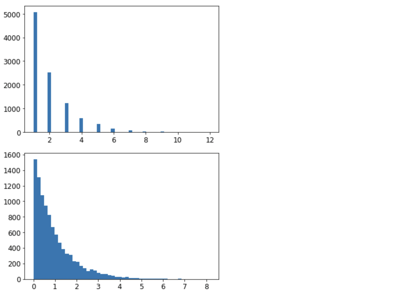
문제
1. loc, iloc 함수의 차이점은?
2. R-squared 값은 무엇이며 이 값이 나타내는 것이 무엇인지 설명하시오
3. 밑의 코드에서는 neg_mean_squared_error를 사용해서 score를 계산하고 있다. 음수를 사용하는 이유가 무엇인지 서술하시오
from sklearn.model_selection import cross_val_score

scores = cross_val_score(tree_reg, housing_prepared, housing_labels,
                         scoring="neg_mean_squared_error", cv=10)
tree_rmse_scores = np.sqrt(-scores)
4. 모델의 추측값의 MSE 값이 0.0이 나왔다는 것은 모델이 완벽하다는 것을 의미한다. (T/F) 또한 자신의 답에 대한 이유를 서술하시오
5. sklearn.svm에서 SVR, SVC를 각각 import한다고 할때 각각의 용도가 무엇인지 서술하시오
6. 다음과 같이 코드를 작성하면 총 몇 번의 훈련이 일어나는지 맞히시오
from sklearn.model_selection import GridSearchCV

param_grid = [
    {'n_estimators': [3, 10], 'max_features': [2, 4, 6, 8, 10]},
    {'bootstrap': [False], 'n_estimators': [3], 'max_features': [2, 3]},
  ]

forest_reg = RandomForestRegressor(random_state=42)

grid_search = GridSearchCV(forest_reg, param_grid, cv=10,
                           scoring='neg_mean_squared_error',
                           return_train_score=True)
grid_search.fit(housing_prepared, housing_labels)